[Article] Can Nuclear War Get You Reelected?

In the 1997 movie Wag the Dog a mysterious consultant played by Robert DeNiro and a Hollywood producer/campaign contributor played by Dustin Hoffman fake a war in Albania complete with a computer generated terrorism video produced by movie biz special effects wizards to divert public attention from a sex scandal engulfing a Bill Clinton-like President who is running for reelection. The phony war succeeds despite several snafus and a brief rebellion by the CIA. The President is reelected amidst a surge of war fever and patriotism. How well do wars work in the real world?

The most spectacular boost in Presidential approval ratings due to a war followed the September 11, 2001 terrorist attacks that killed about 3,000 people on US soil, probably the largest single day massacre in US history both in absolute numbers and fraction of the population. (The few day Santee massacre of settlers by Dakota Sioux Indians in Minnesota in 1862 probably killed a larger fraction of the population at the time.) President George W. Bush and the Republicans seem to have benefited electorally from the subsequent “war on terror” in the 2002 and 2004 elections.

However, historically the effect of wars and national security events such as the successful launch of the Sputnik I (October 4, 1957) and II (November 3, 1957) satellites by the Soviet Union on Presidential approval ratings and electoral prospects is much more varied. Sputnik II is significant because the second satellite was large enough to carry a nuclear bomb unlike the beach ball sized Sputnik I.

Truman and the Korean War

President Harry Truman’s approval ratings had been declining for over a year prior to the start of the Korean War. He may have experienced a slight bump for a couple of months (see plot above) followed by further decline.

Eisenhower and the End of the Korean War

Like most new Presidents, Dwight Eisenhower experienced a big “honeymoon” jump over his predecessor Harry Truman. There is little sign he either benefited or suffered from the end of the Korean War.

Eisenhower and Sputnik I and II

Eisenhower’s approval ratings had been declining for almost a year when the Soviet Union successfully launched the first satellite Sputnik I on October 4, 1957. This was followed by the much larger Sputnik II on November 3, 1957 — theoretically capable of carrying a nuclear bomb. Although Sputnik I and II were big news stories and led to a huge reaction in the United States, there is no clear effect on Eisenhower’s approval ratings. He rebounded in early 1958 and left office as one of the most popular Presidents.

However, Eisenhower, his administration, and his Vice President Richard Nixon who ran for President in 1960 were heavily criticized over the missile race with the Soviet Union due to Sputnik. Sputnik was followed by high profile, highly publicized failures of US attempts to launch satellites. Administration claims that the Soviet Union was in fact behind the US in the race to build nuclear missiles were widely discounted, although this seems to have been true.

John F. Kennedy ran successfully for President in 1960 claiming the notorious “missile gap” and calling for a massive nuclear missile build up, winning narrowly over Nixon in a bitterly contested election with widespread allegations of voting fraud in Texas and Chicago. Eisenhower’s famous farewell address coining (or at least popularizing) the phrase “military industrial complex” was a reaction to the controversy over Sputnik and the nuclear missile program.

Kennedy and the Cuban Missile Crisis

President Kennedy experienced a large boost in previously declining approval ratings during and after the Cuban Missile Crisis in October of 1962. This is often considered the closest the world has come to a nuclear war until the recent confrontation with Russia over the Ukraine. It also occurred only weeks before the mid-term elections in November of 1962.

Johnson and the Vietnam War

The Vietnam War ultimately destroyed President Lyndon Johnson’s approval ratings with the aging President declining to run for another term in 1968 amidst massive protests and challenges from Senator Robert Kennedy and others. There is actually little evidence of a boost from the Gulf of Tonkin incidents in August of 1964 and the subsequent Gulf of Tonkin resolution leading to the larger war.

President Johnson ran on a “peace” platform, successfully portraying the Republican candidate Senator Barry Goldwater of Arizona as a nutcase warmonger. Yet, Johnson — at the same time — visibly escalated the US involvement in the then obscure nation of Vietnam in August only a few months before the Presidential election in 1964.

Ford and the End of the Vietnam War

The end of the Vietnam War (April 30, 1975) seems to have boosted President Gerald Ford’s approval ratings significantly, about ten percent. Nonetheless, he was defeated by Jimmy Carter in 1976.

Carter and the Iran Hostage Crisis

President Jimmy Carter experienced a substantial boost in approval ratings when “students” took over the US Embassy in Tehran, Iran on November 4, 1979, holding the embassy staff hostage for 444 days. This lasted a few months, followed by a rapid decline back to Carter’s previous dismal approval ratings. The failure to rescue or secure the release of the hostages almost certainly contributed to Carter’s loss the Ronald Reagan in 1980.

George H.W. Bush and Iraq War I (Operation Desert Storm)

President George Herbert Walker Bush experienced a large boost in approval ratings at the end of the first Iraq War followed by a large and rapid decline, losing to Bill Clinton in 1992.

President George Bush, September 11, Iraq War II, and Afghanistan are discussed at the start of this article — overall probably the clearest boost in approval and electoral performance from a war at least since World War II.

Biden and Ukraine

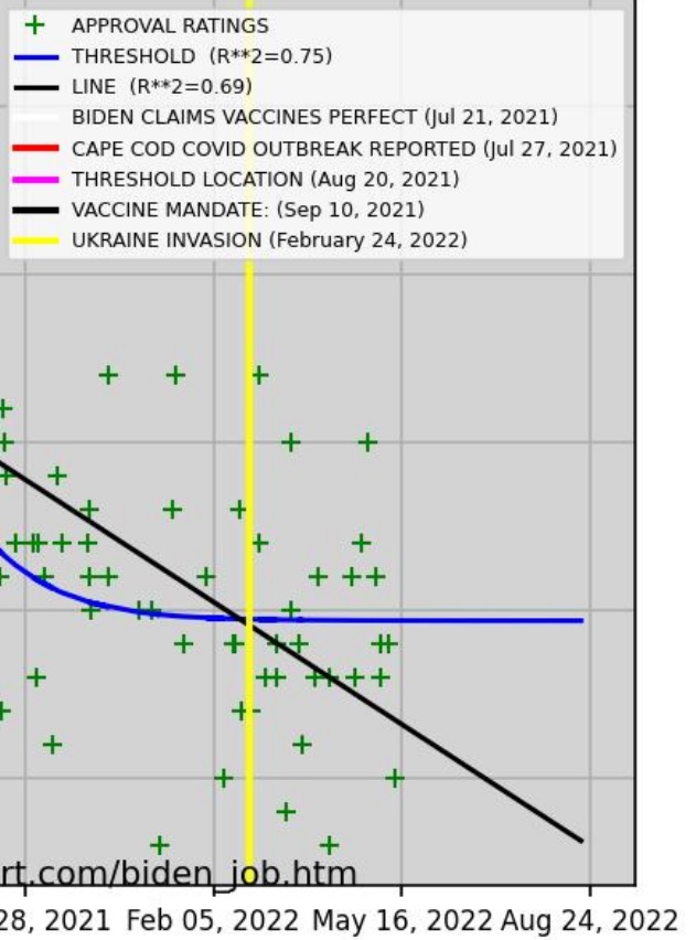
As of June 16, 2022, President Joe Biden’s approval ratings have continued to decline since the February 24, 2022 invasion of Ukraine by Russia. There is not the slightest sign of any boost.

Conclusion

Despite the folk tradition epitomized by the movie Wag the Dog that wars boost a President’s approval and electoral prospects — at least initially — history shows mixed results. Some wars have clearly boosted the President’s prospects, notably after September 11, and others have done nothing or even contributed to further decline. Korea, for example, seems to have only contributed to President Truman’s marked decline and the loss to Eisenhower in 1952.

Probably the lesson is to avoid wars and focus on resolving substantive domestic economic problems.

(C) 2022 by John F. McGowan, Ph.D.

About Me

John F. McGowan, Ph.D. solves problems using mathematics and mathematical software, including developing gesture recognition for touch devices, video compression and speech recognition technologies. He has extensive experience developing software in C, C++, MATLAB, Python, Visual Basic and many other programming languages. He has been a Visiting Scholar at HP Labs developing computer vision algorithms and software for mobile devices. He has worked as a contractor at NASA Ames Research Center involved in the research and development of image and video processing algorithms and technology. He has published articles on the origin and evolution of life, the exploration of Mars (anticipating the discovery of methane on Mars), and cheap access to space. He has a Ph.D. in physics from the University of Illinois at Urbana-Champaign and a B.S. in physics from the California Institute of Technology (Caltech).

[Video] Why Did Biden’s Approval Crash in August 2021?

Uncensored Video: Odysee NewTube ARCHIVE BitChute

Twelve minute video on why President Biden’s approval ratings crashed in August of 2021.

References:

https://www.pbs.org/newshour/show/older-americans-make-up-a-majority-of-covid-deaths-they-are-falling-behind-on-boosters

https://www.npr.org/2022/02/19/1081948849/elderly-people-make-up-75-of-covid-19-deaths-partially-due-to-loneliness

https://web.archive.org/web/20210731120830/https://covid.cdc.gov/covid-data-tracker/#datatracker-home

https://gis.cdc.gov/grasp/fluview/mortality.html

https://www.cnn.com/2021/07/22/politics/fact-check-biden-cnn-town-hall-july/index.html

Jefferson’s First Inaugural Address: https://avalon.law.yale.edu/19th_century/jefinau1.asp

About Us:

Main Web Site: https://mathematical-software.com/
Censored Search: https://censored-search.com/
A search engine for censored Internet content. Find the answers to your problems censored by advertisers and other powerful interests!

Subscribe to our free Weekly Newsletter for articles and videos on practical mathematics, Internet Censorship, ways to fight back against censorship, and other topics by sending an email to: subscribe [at] mathematical-software.com

Avoid Internet Censorship by Subscribing to Our RSS News Feed: http://wordpress.jmcgowan.com/wp/feed/

Legal Disclaimers: http://wordpress.jmcgowan.com/wp/legal/

Support Us:
PATREON: https://www.patreon.com/mathsoft
SubscribeStar: https://www.subscribestar.com/mathsoft

BitChute (Video): https://www.bitchute.com/channel/HGgoa2H3WDac/
Brighteon (Video): https://www.brighteon.com/channels/mathsoft
Odysee (Video): https://odysee.com/@MathematicalSoftware:5
NewTube (Video): https://newtube.app/user/mathsoft
Archive (Video): https://archive.org/details/@mathsoft

(C) 2022 by John F. McGowan, Ph.D.

About Me

John F. McGowan, Ph.D. solves problems using mathematics and mathematical software, including developing gesture recognition for touch devices, video compression and speech recognition technologies. He has extensive experience developing software in C, C++, MATLAB, Python, Visual Basic and many other programming languages. He has been a Visiting Scholar at HP Labs developing computer vision algorithms and software for mobile devices. He has worked as a contractor at NASA Ames Research Center involved in the research and development of image and video processing algorithms and technology. He has published articles on the origin and evolution of life, the exploration of Mars (anticipating the discovery of methane on Mars), and cheap access to space. He has a Ph.D. in physics from the University of Illinois at Urbana-Champaign and a B.S. in physics from the California Institute of Technology (Caltech).

[Article] A First Look at Presidential Approval Ratings with Math Recognition

This article takes a first look at historical Presidential approval ratings (approval polls from Gallup and other polling services) from Harry Truman through Joe Biden using our math recognition and automated model fitting technology. Our Math Recognition (MathRec) engine has a large, expanding database of known mathematics and uses AI and pattern recognition technology to identify likely candidate mathematical models for data such as the Presidential Approval ratings data. It then automatically fits these models to the data and provides a ranked list of models ordered by goodness of fit, usually the coefficient of determination or “R Squared” metric. It automates, speeds up, and increases the accuracy of data analysis — finding actionable predictive models for data.

The plots show a model — the blue lines — which “predicts” the approval rating based on unemployment rate (UNRATE), the real inflation adjusted value of gold, and time after the first inauguration of a US President — the so-called honeymoon period. The model “explains” about forty-three (43%) of the variation in the approval ratings. This is the “R Squared” or coefficient of determination for the model. The model has a correlation of about sixty-six percent (0.66) with the actual Presidential approval ratings. Note that a model can have a high correlation with data and yet the coefficient of determination is small.

One might expect US Presidential approval ratings to decline with increasing unemployment and/or an increase in the real value of gold reflecting uncertainty and anxiety over the economy. It is generally thought that new Presidents experience a honeymoon period after first taking office. This seems supported by the historical data, suggesting a honeymoon of about six months — with the possible exception of President Trump in 2017.

The model does not (yet) capture a number of notable historical events that appear to have significantly boosted or reduced the US Presidential approval ratings: the Cuban Missile crisis, the Iran Hostage Crisis, the September 11 attacks, the Watergate scandal, and several others. Public response to dramatic events such as these is variable and hard to predict or model. The public often seems to rally around the President at first and during the early stages of a war, but support may decline sharply as a war drags on and/or serious questions arise regarding the war.

There are, of course, a number of caveats on the data. Presidential approval polls empirically vary by several percentage points today between different polling services. There are several historical cases where pre-election polling predictions were grossly in error including the 2016 US Presidential election. A number of polls called the Dewey-Truman race in 1948 wrong, giving rise to the famous photo of President Truman holding up a copy of the Chicago Tribune announcing Dewey’s election victory.

The input data is from the St. Louis Federal Reserve Federal Reserve Economic Data (FRED) web site, much of it from various government agencies such as unemployment data from the Bureau of Labor Statistics. There is a history of criticism of these numbers. Unemployment and inflation rate numbers often seem lower than my everyday experience. As noted, a number of economists and others have questioned the validity of federal unemployment, inflation and price level, and other economic numbers.

(C) 2022 by John F. McGowan, Ph.D.

About Me

John F. McGowan, Ph.D. solves problems using mathematics and mathematical software, including developing gesture recognition for touch devices, video compression and speech recognition technologies. He has extensive experience developing software in C, C++, MATLAB, Python, Visual Basic and many other programming languages. He has been a Visiting Scholar at HP Labs developing computer vision algorithms and software for mobile devices. He has worked as a contractor at NASA Ames Research Center involved in the research and development of image and video processing algorithms and technology. He has published articles on the origin and evolution of life, the exploration of Mars (anticipating the discovery of methane on Mars), and cheap access to space. He has a Ph.D. in physics from the University of Illinois at Urbana-Champaign and a B.S. in physics from the California Institute of Technology (Caltech).

[Video] How to Analyze Data Using a Baseline Linear Model in Python

https://www.bitchute.com/video/b1D2KMk4kGKH/

Other Uncensored Video Links: NewTube Odysee

YouTube

Video on how to analyze data using a baseline linear model in the Python programming language. A baseline linear model is often a good starting point, reference for developing and evaluating more advanced usually non-linear models of data.

Article with source code: http://wordpress.jmcgowan.com/wp/article-how-to-analyze-data-with-a-baseline-linear-model-in-python/

(C) 2022 by John F. McGowan, Ph.D.

About Me

John F. McGowan, Ph.D. solves problems using mathematics and mathematical software, including developing gesture recognition for touch devices, video compression and speech recognition technologies. He has extensive experience developing software in C, C++, MATLAB, Python, Visual Basic and many other programming languages. He has been a Visiting Scholar at HP Labs developing computer vision algorithms and software for mobile devices. He has worked as a contractor at NASA Ames Research Center involved in the research and development of image and video processing algorithms and technology. He has published articles on the origin and evolution of life, the exploration of Mars (anticipating the discovery of methane on Mars), and cheap access to space. He has a Ph.D. in physics from the University of Illinois at Urbana-Champaign and a B.S. in physics from the California Institute of Technology (Caltech).

[Article] How to Analyze Data with a Baseline Linear Model in Python

This article shows Python programming language source code to perform a simple linear model analysis of time series data. Most real world data is not linear but a linear model provides a common baseline starting point for comparison of more advanced, generally non-linear models.

Simulated Nearly Linear Data with Linear Model
"""
Standalone linear model example code.

Generate simulated data and fit model to this simulated data.

LINEAR MODEL FORMULA:

OUTPUT = MULT_T*DATE_TIME + MULT_1*INPUT_1 + MULT_2*INPUT_2 + CONSTANT + NOISE

set MULT_T to 0.0 for simulated data.  Asterisk * means MULTIPLY
from grade school arithmetic.  Python and most programming languages
use * to indicate ordinary multiplication.

(C) 2022 by Mathematical Software Inc.

Point of Contact (POC): John F. McGowan, Ph.D.
E-Mail: ceo@mathematical-software.com

"""

# Python Standard Library
import os
import sys
import time
import datetime
import traceback
import inspect
import glob
# Python add on modules
import numpy as np  # NumPy
import pandas as pd  # Python Data Analysis Library
import matplotlib.pyplot as plt  # MATLAB style plotting
from sklearn.metrics import r2_score  # scikit-learn
import statsmodels.api as sm  # OLS etc.

# STATSMODELS
#
# statsmodels is a Python module that provides classes and functions for
# the estimation of many different statistical models, as well as for
# conducting statistical tests, and statistical data exploration. An
# extensive list of result statistics are available for each
# estimator. The results are tested against existing statistical
# packages to ensure that they are correct. The package is released
# under the open source Modified BSD (3-clause) license.
# The online documentation is hosted at statsmodels.org.
#
# statsmodels supports specifying models using R-style formulas and pandas DataFrames. 


def debug_prefix(stack_index=0):
    """
    return <file_name>:<line_number> (<function_name>)

    REQUIRES: import inspect
    """
    the_stack = inspect.stack()
    lineno = the_stack[stack_index + 1].lineno
    filename = the_stack[stack_index + 1].filename
    function = the_stack[stack_index + 1].function
    return (str(filename) + ":"
            + str(lineno)
            + " (" + str(function) + ") ")  # debug_prefix()


def is_1d(array_np,
          b_trace=False):
    """
    check if array_np is 1-d array

    Such as array_np.shape:  (n,), (1,n), (n,1), (1,1,n) etc.

    RETURNS: True or False

    TESTING: Use DOS> python -c "from standalone_linear import *;test_is_1d()"
    to test this function.

    """
    if not isinstance(array_np, np.ndarray):
        raise TypeError(debug_prefix() + "argument is type "
                        + str(type(array_np))
                        + " Expected np.ndarray")

    if array_np.ndim == 1:
        # array_np.shape == (n,)
        return True
    elif array_np.ndim > 1:
        # (2,3,...)-d array
        # with only one axis with more than one element
        # such as array_np.shape == (n, 1) etc.
        #
        # NOTE: np.array.shape is a tuple (not a np.ndarray)
        # tuple does not have a shape
        #
        if b_trace:
            print("array_np.shape:", array_np.shape)
            print("type(array_np.shape:",
                  type(array_np.shape))
            
        temp = np.array(array_np.shape)  # convert tuple to np.array
        reference = np.ones(temp.shape, dtype=int)

        if b_trace:
            print("reference:", reference)

        mask = np.zeros(temp.shape, dtype=bool)
        for index, value in enumerate(temp):
            if value == 1:
                mask[index] = True

        if b_trace:
            print("mask:", mask)
        
        # number of axes with one element
        axes = temp[mask]
        if isinstance(axes, np.ndarray):
            n_ones = axes.size
        else:
            n_ones = axes
            
        if n_ones >= (array_np.ndim - 1):
            return True
        else:
            return False
    # END is_1d(array_np)


def test_is_1d():
    """
    test is_1d(array_np) function  works
    """

    assert is_1d(np.array([1, 2, 3]))
    assert is_1d(np.array([[10, 20, 33.3]]))
    assert is_1d(np.array([[1.0], [2.2], [3.34]]))
    assert is_1d(np.array([[[1.0], [2.2], [3.3]]]))
    
    assert not is_1d(np.array([[1.1, 2.2], [3.3, 4.4]]))

    print(debug_prefix(), "PASSED")
    # test_is_1d()


def is_time_column(column_np):
    """
    check if column_np is consistent with a time step sequence
    with uniform time steps. e.g. [0.0, 0.1, 0.2, 0.3,...]

    ARGUMENT: column_np -- np.ndarray with sequence

    RETURNS: True or False
    """
    if not isinstance(column_np, np.ndarray):
        raise TypeError(debug_prefix() + "argument is type "
                        + str(type(column_np))
                        + " Expected np.ndarray")

    if is_1d(column_np):
        # verify if time step sequence is nearly uniform
        # sequence of time steps such as (0.0, 0.1, 0.2, ...)
        #
        delta_t = np.zeros(column_np.size-1)
        for index, tval in enumerate(column_np.ravel()):
            if index > 0:
                previous_time = column_np[index-1]
                if tval > previous_time:
                    delta_t[index-1] = tval - previous_time
                else:
                    return False

        # now check that time steps are almost the same
        delta_t = np.median(delta_t)
        delta_range = np.max(delta_t) - np.min(delta_t)
        delta_pct = delta_range / delta_t
        
        print(debug_prefix(),
              "INFO: delta_pct is:", delta_pct, flush=True)
        
        if delta_pct > 1e-6:
            return False
        else:
            return True  # steps are almost the same
    else:
        raise ValueError(debug_prefix() + "argument has more"
                         + " than one (1) dimension.  Expected 1-d")
    # END is_time_column(array_np)


def validate_time_series(time_series):
    """
    validate a time series NumPy array

    Should be a 2-D NumPy array (np.ndarray) of float numbers

    REQUIRES: import numpy as np

    """
    if not isinstance(time_series, np.ndarray):
        raise TypeError(debug_prefix(stack_index=1)
                        + " time_series is type "
                        + str(type(time_series))
                        + " Expected np.ndarray")

    if not time_series.ndim == 2:
        raise TypeError(debug_prefix(stack_index=1)
                        + " time_series.ndim is "
                        + str(time_series.ndim)
                        + " Expected two (2).")

    for row in range(time_series.shape[0]):
        for col in range(time_series.shape[1]):
            value = time_series[row, col]
            if not isinstance(value, np.float64):
                raise TypeError(debug_prefix(stack_index=1)
                                + "time_series[" + str(row)
                                + ", " + str(col) + "] is type "
                                + str(type(value))
                                + " expected float.")

    # check if first column is a sequence of nearly uniform time steps
    #
    if not is_time_column(time_series[:, 0]):
        raise TypeError(debug_prefix(stack_index=1)
                        + "time_series[:, 0] is not a "
                        + "sequence of nearly uniform time steps.")

    return True  # validate_time_series(...)


def fit_linear_to_time_series(new_series):
    """
    Fit multivariate linear model to data.  A wrapper
    for ordinary least squares (OLS).  Include possibility
    of direct linear dependence of the output on the date/time.
    Mathematical formula:

    output = MULT_T*DATE_TIME + MULT_1*INPUT_1 + ... + CONSTANT

    ARGUMENTS: new_series -- np.ndarray with two dimensions
                             with multivariate time series.
                             Each column is a variable.  The
                             first column is the date/time
                             as a float value, usually a
                             fractional year.  Final column
                             is generally the suspected output
                             or dependent variable.

                             (time)(input_1)...(output)

    RETURNS: fitted_series -- np.ndarray with two dimensions
                              and two columns: (date/time) (output
                              of fitted model)

             results --
                 statsmodels.regression.linear_model.RegressionResults

    REQUIRES: import numpy as np
              import pandas as pd
              import statsmodels.api as sm  # OLS etc.

    (C) 2022 by Mathematical Software Inc.

    """
    validate_time_series(new_series)

    #
    # a data frame is a package for a set of numbers
    # that includes key information such as column names,
    # units etc.
    #
    input_data_df = pd.DataFrame(new_series[:, :-1])
    input_data_df = sm.add_constant(input_data_df)

    output_data_df = pd.DataFrame(new_series[:, -1])

    # statsmodels Ordinary Least Squares (OLS)
    model = sm.OLS(output_data_df, input_data_df)
    results = model.fit()  # fit linear model to the data
    print(results.summary())  # print summary of results
                              # with fit parameters, goodness
                              # of fit statistics etc.

    # compute fitted model values for comparison to data
    #
    fitted_values_df = results.predict(input_data_df)

    fitted_series = np.vstack((new_series[:, 0],
                               fitted_values_df.values)).transpose()

    assert fitted_series.shape[1] == 2, \
        str(fitted_series.shape[1]) + " columns, expected two(2)."

    validate_time_series(fitted_series)

    return fitted_series, results  # fit_linear_to_time_series(...)


def test_fit_linear_to_time_series():
    """
    simple test of fitting  a linear model to simple
    simulated data.

    ACTION: Displays plot comparing data to the linear model.

    REQUIRES: import numpy as np
              import matplotlib.pyplot as plt
              from sklearn.metrics impor r2_score (scikit-learn)

    NOTE: In mathematics a function f(x) is linear if:

    f(x + y) = f(x) + f(y)  # function of sum of two inputs
                            # is sum of function of each input value

    f(a*x) = a*f(x)         # function of constant multiplied by
                            # an input is the same constant
                            # multiplied by the function of the
                            # input value

    (C) 2022 by Mathematical Software Inc.
    """

    # simulate monthly data for years 2010 to 2021
    time_steps = np.linspace(2010.0, 2022.0, 120)
    #
    # set random number generator "seed"
    #
    np.random.seed(375123)  # make test reproducible
    # make random walks for the input values
    input_1 = np.cumsum(np.random.normal(size=time_steps.shape))
    input_2 = np.cumsum(np.random.normal(size=time_steps.shape))

    # often awe inspiring Greek letters (alpha, beta,...)
    mult_1 = 1.0  # coefficient or multiplier for input_1
    mult_2 = 2.0   # coefficient or multiplier for input_2
    constant = 3.0  # constant value  (sometimes "pedestal" or "offset")

    # simple linear model
    output = mult_1*input_1 + mult_2*input_2 + constant
    # add some simulated noise
    noise = np.random.normal(loc=0.0,
                             scale=2.0,
                             size=time_steps.shape)

    output = output + noise

    # bundle the series into a single multivariate time series
    data_series = np.vstack((time_steps,
                             input_1,
                             input_2,
                             output)).transpose()

    #
    # np.vstack((array1, array2)) vertically stacks
    # array1 on top of array 2:
    #
    #  (array 1)
    #  (array 2)
    #
    # transpose() to convert rows to vertical columns
    #
    # data_series has rows:
    #    (date_time, input_1, input_2, output)
    #    ...
    #

    # the model fit will estimate the values for the
    # linear model parameters MULT_T, MULT_1, and MULT_2

    fitted_series, \
        fit_results = fit_linear_to_time_series(data_series)

    assert fitted_series.shape[1] == 2, "wrong number of columns"

    model_output = fitted_series[:, 1].flatten()

    #
    # Is the model "good enough" for practical use?
    #
    # Compure R-SQUARED also known as R**2
    # coefficient of determination, a goodness of fit measure
    # roughly percent agreement between data and model
    #
    r2 = r2_score(output,  # ground truth / data
                  model_output  # predicted values
                  )

    #
    # Plot data and model predictions
    #

    model_str = "OUTPUT = MULT_1*INPUT_1 + MULT_2*INPUT_2 + CONSTANT"

    f1 = plt.figure()
    # set light gray background for plot
    # must do this at start after plt.figure() call for some
    # reason
    #
    ax = plt.axes()  # get plot axes
    ax.set_facecolor("lightgray")  # confusingly use set_facecolor(...)
    # plt.ylim((ylow, yhi))  # debug code
    plt.plot(time_steps, output, 'g+', label='DATA')
    plt.plot(time_steps, model_output, 'b-', label='MODEL')
    plt.plot(time_steps, data_series[:, 1], 'cd', label='INPUT 1')
    plt.plot(time_steps, data_series[:, 2], 'md', label='INPUT 2')
    plt.suptitle(model_str)
    plt.title(f"Simple Linear Model (R**2={100*r2:.2f}%)")

    ax.text(1.05, 0.5,
            model_str,
            rotation=90, size=7, weight='bold',
            ha='left', va='center', transform=ax.transAxes)

    ax.text(0.01, 0.01,
            debug_prefix(),
            color='black',
            weight='bold',
            size=6,
            transform=ax.transAxes)

    ax.text(0.01, 0.03,
            time.ctime(),
            color='black',
            weight='bold',
            size=6,
            transform=ax.transAxes)

    plt.xlabel("YEAR FRACTION")
    plt.ylabel("OUTPUT")
    plt.legend(fontsize=8)
    # add major grid lines
    plt.grid()
    plt.show()

    image_file = "test_fit_linear_to_time_series.jpg"
    if os.path.isfile(image_file):
        print("WARNING: removing old image file:",
              image_file)
        os.remove(image_file)

    f1.savefig(image_file,
               dpi=150)

    if os.path.isfile(image_file):
        print("Wrote plot image to:",
              image_file)

    # END test_fit_linear_to_time_series()


if __name__ == "__main__":
    # MAIN PROGRAM

    test_fit_linear_to_time_series()  # test linear model fit

    print(debug_prefix(), time.ctime(), "ALL DONE!")

(C) 2022 by John F. McGowan, Ph.D.

About Me

John F. McGowan, Ph.D. solves problems using mathematics and mathematical software, including developing gesture recognition for touch devices, video compression and speech recognition technologies. He has extensive experience developing software in C, C++, MATLAB, Python, Visual Basic and many other programming languages. He has been a Visiting Scholar at HP Labs developing computer vision algorithms and software for mobile devices. He has worked as a contractor at NASA Ames Research Center involved in the research and development of image and video processing algorithms and technology. He has published articles on the origin and evolution of life, the exploration of Mars (anticipating the discovery of methane on Mars), and cheap access to space. He has a Ph.D. in physics from the University of Illinois at Urbana-Champaign and a B.S. in physics from the California Institute of Technology (Caltech).

[Video] How to Extract Data from Images of Plots

Free Speech Video Links: Odysee RUMBLE NewTube

Short video on how to extract data from images of plots using WebPlotDigitizer, a free, open-source program available for Windows, Mac OS X, and Linux platforms.

WebPlotDigitizer web site: https://automeris.io/WebPlotDigitizer/

(C) 2022 by John F. McGowan, Ph.D.

About Me

John F. McGowan, Ph.D. solves problems using mathematics and mathematical software, including developing gesture recognition for touch devices, video compression and speech recognition technologies. He has extensive experience developing software in C, C++, MATLAB, Python, Visual Basic and many other programming languages. He has been a Visiting Scholar at HP Labs developing computer vision algorithms and software for mobile devices. He has worked as a contractor at NASA Ames Research Center involved in the research and development of image and video processing algorithms and technology. He has published articles on the origin and evolution of life, the exploration of Mars (anticipating the discovery of methane on Mars), and cheap access to space. He has a Ph.D. in physics from the University of Illinois at Urbana-Champaign and a B.S. in physics from the California Institute of Technology (Caltech).

[Video] How to Analyze Simple Data Using Python

Uncensored Video Links: BitChute NewTube ARCHIVE Brighteon Odysee

Video on how to analyze simple data using the Python programming language using President Biden’s approval ratings as an example.

(C) 2022 by John F. McGowan, Ph.D.

About Me

John F. McGowan, Ph.D. solves problems using mathematics and mathematical software, including developing gesture recognition for touch devices, video compression and speech recognition technologies. He has extensive experience developing software in C, C++, MATLAB, Python, Visual Basic and many other programming languages. He has been a Visiting Scholar at HP Labs developing computer vision algorithms and software for mobile devices. He has worked as a contractor at NASA Ames Research Center involved in the research and development of image and video processing algorithms and technology. He has published articles on the origin and evolution of life, the exploration of Mars (anticipating the discovery of methane on Mars), and cheap access to space. He has a Ph.D. in physics from the University of Illinois at Urbana-Champaign and a B.S. in physics from the California Institute of Technology (Caltech).

[Video] How to Analyze Simple Data with Libre Office Calc

Uncensored Video Links: BitChute NewTube

Video on how to perform a simple analysis of simple data in LibreOffice Calc, a free open-source “clone” of Microsoft Excel. Demonstrates how to use the Trend Line feature in LibreOffice Calc Charts. Discusses how to use the R Squared goodness of fit statistic to evaluate the analysis.

(C) 2022 by John F. McGowan, Ph.D.

About Me

John F. McGowan, Ph.D. solves problems using mathematics and mathematical software, including developing gesture recognition for touch devices, video compression and speech recognition technologies. He has extensive experience developing software in C, C++, MATLAB, Python, Visual Basic and many other programming languages. He has been a Visiting Scholar at HP Labs developing computer vision algorithms and software for mobile devices. He has worked as a contractor at NASA Ames Research Center involved in the research and development of image and video processing algorithms and technology. He has published articles on the origin and evolution of life, the exploration of Mars (anticipating the discovery of methane on Mars), and cheap access to space. He has a Ph.D. in physics from the University of Illinois at Urbana-Champaign and a B.S. in physics from the California Institute of Technology (Caltech).

[Book Review] Unmasked by Ian Miller

Unmasked: The Global Failure of COVID Mask Mandates

By Ian Miller

Post Hill Press, New York, 2022

Unmasked is an easy-to-read graph-filled book that makes a very strong case that masks, also known as face coverings, have little or no effect on infection, transmission, hospitalization or death due to COVID-19 and may even be somewhat harmful. Although the book does not quantify what “little” might mean, one of several weaknesses of the book, it likely means at most a few percent reduction. After nearly two years of COVID-19 and masking, this should be pretty obvious and non-controversial, but it remains a highly contentious topic with the United States CDC continuing to produce and promote dubious mask studies claiming or implying high levels of mask effectiveness. Conservative commentator Dan Bongino was recently deplatformed by YouTube (Google/Alphabet) ostensibly for asserting that masks don’t work (or cloth masks don’t work according to some accounts).

The book discusses how the “settled science” before the end of March 2020 was that masks had little or no benefit as shown by many prior studies. Masks had in fact clearly failed during the infamous 1918 influenza epidemic. This was reflected in now infamous public statements by Anthony Fauci, US Surgeon General Jerome Adams, and other “experts.” The “settled science” reversed one-hundred and eighty degrees at the beginning of April 2020 with Fauci subsequently claiming his original statements were a lie, now usually described as a “noble lie” to save N95 masks for health care workers.

The book devotes several short readable chapters to masks and the flu (meaning the influenza virus), the CDC pro-mask studies, the US states California and Florida arguably representing the two extremes on mask policy, Sweden which largely eschewed masks, and international comparisons.

The climax of the book is a long, dense chapter going alphabetically through all US states and Washington DC, with a graph of daily new cases per million population for each jurisdiction during the pandemic, graphs annotated with start and stop dates of mask mandates, a few measurements of mask compliance rates, and notable news articles either extolling the mask policy in the state shortly before cases skyrocketed or predicting disaster following removal of a mask mandate, followed by continuing sharp drops in the daily new cases.

The chapter closes with a bar chart showing age adjusted death rates for all US states (no Washington D.C.) sourced in tiny almost unreadable type to the US CDC, from the highest age adjusted death rate (New Jersey with about 140 COVID deaths per one-hundred thousand residents) to the lowest (Vermont with about 15 deaths per one-hundred thousand). States without mask mandates or minimal mask mandates are highlighted, spanning nearly the entire range with South Dakota as 3rd worst state just behind Number 2 New York and Alaska at 46. High profile Florida falls at forty in the graph with about 55 deaths per one-hundred thousand. This is for the twelve month period thru the fourth quarter (Q4) of 2020.

The plots and other data in the book make a strong case that masks at best only have a small positive effect that must nearly always be swamped out by other factors which the book largely does not discuss.

Several Weaknesses

The book appears to be largely aimed at conservative, libertarian, pro-Trump or anti-(anti-Trump) audiences. By anti-(anti-Trump) is meant the many people who fall somewhere between unenthused about Trump to quite concerned but view the “get Trump at any cost” reaction to Trump as a dangerous, irrational overreaction. The anti-(anti-Trumpers) span the conventional political spectrum and arguably include such prominent figures as Glenn Greenwald, former Rolling Stone writer Matt Taibbi, and podcaster Joe Rogan. The book features advanced praise quotes from libertarian author Tom Woods, conservative commentator Ann Coulter, and similar figures on its first page.

While the book does have references, these are all or nearly all popular news articles and not scholarly peer reviewed scientific journal articles of which their are many, pre-prints, or similar non-peer reviewed content (e.g. “working papers”). The numerous plots do have a reference in tiny print at the bottom, almost unreadable. These references are often secondary sources such as Worldometer or the New York Times COVID dashboards etc. This is better than Scot Atlas’s A Plague Upon Our House, also from Post Hill Press, which has no references despite the author emphasizing the importance of scientific references in critiquing Anthony Fauci and others. However, the book should have scholarly references and links to primary data sources such as the CDC web site.

The plots are quite small. The printed book is about 5 1/2 inches wide by 8 1/4 inches high with nearly all plots about 4 inches wide by 2 1/2 inches high with small to very tiny type, undoubtedly hard for many readers. It probably would have been better to devote an entire page to each plot for clarity.

The book should devote more space to the issue of mask compliance. Quite clearly the mask mandates failed, but the fallback argument is that the people, especially knuckle dragging Trump supporters, failed to follow the mask mandates. The book does cite several studies of mask compliance — actual mask wearing — contradicting this explanation. Living in the San Francisco Bay Area, I am personally sure mask compliance was high in the SF Bay Area and likely other urban centers such as LA and San Diego. But even in California, the failure could be blamed on rural Californians. In fact, COVID-19 deaths soared in urban Santa Clara County during the winter of 2020-2021 despite the heavy use of masks.

COVID-19 Deaths in Santa Clara County (SF Bay Area/Silicon Valley)

The weakest part of the book is the fourth chapter on the CDC’s handful of highly promoted studies claiming or implying dramatic benefits from mask wearing. These are of course highly contradicted by the mountain of data in the final chapter as well as other chapters. Nonetheless some of the arguments seemed rather weak relying on typical assertions made during scientific and political controversies. Accusations of “poor scientific or statistical methodology” are common and need to be specifically backed up.

The book would be stronger with a chapter on why masks might fail. The likely explanation is that there is practically significant aerosol transmission of COVID-19, meaning the virus floats in the air like fine dust or smoke. The viral particles are tiny, too small to be seen by an optical microscope, about 1/500th the width of a human hair. They can easily flow through the mesh of cloth or surgical masks. The N95 masks claim to stop 95 percent of particles 0.3 microns (300 nm) in diameter. The coronavirus is about 0.14 micron (140 nm) in diameter. The N95 masks probably stop less than 95 percent of such small particles. In theory even one viable viral particle can infect and kill a person.

The book would also benefit from a chapter on the downsides of masks which reduce air intake, trap carbon dioxide, interfere with communication, and have other negative effects. Masks are not advised for persons with asthma and various other respiratory problems. How well can we determine who can safely wear a mask and for how long. OSHA has strict limits on mask use in work settings that would preclude the use of masks to try to control COVID-19.

The book would be stronger by quantifying the bounds on the effectiveness of masks and discussing under what conditions these quantitative bounds apply. This is likely to be a range from negative a few percent (makes things worse) to positive a few percent (weak benefit).

Some articles that review the primary scientific literature in more and better detail than Unmasked are:

“Do Masks Work?” by Jeffrey H. Anderson, City Journal, August 11, 2021

More than 150 Comparative Studies and Articles on Mask Ineffectiveness and Harms by Paul Elias Alexander, (libertarian) Brownstone Institute, December 20, 2021

“Masks don’t work” by Denis Rancourt

Mask studies reach a new scientific low point,” by Vinay Prasad, Brownstone Institute, Feb. 6, 2022

All have some weaknesses and suffer from the politicization of the mask issue in various ways, but overall complement the weaknesses of Unmasked.

At this point, with huge numbers of fully vaccinated, mask wearing persons contracting the Omicron variant or at least getting sick and getting test results interpreted as Omicron, it should be clear that masks are largely ineffective, just as was the case during the 1918 influenza epidemic. Rather than beating a dead horse, public discussion and efforts to mitigate the COVID-19 pandemic should focus on more promising options such as UV lighting in ducts and ventilation systems, installation of air purifiers with UV sub-systems to kill viral particles in the air, as well as other possibilities which avoid the enormous social and psychological costs, not to mention physical health risks of prolonged mask wearing.

(C) 2022 by John F. McGowan, Ph.D.

About Me

John F. McGowan, Ph.D. solves problems using mathematics and mathematical software, including developing gesture recognition for touch devices, video compression and speech recognition technologies. He has extensive experience developing software in C, C++, MATLAB, Python, Visual Basic and many other programming languages. He has been a Visiting Scholar at HP Labs developing computer vision algorithms and software for mobile devices. He has worked as a contractor at NASA Ames Research Center involved in the research and development of image and video processing algorithms and technology. He has published articles on the origin and evolution of life, the exploration of Mars (anticipating the discovery of methane on Mars), and cheap access to space. He has a Ph.D. in physics from the University of Illinois at Urbana-Champaign and a B.S. in physics from the California Institute of Technology (Caltech).

[Book Review] Pandemia by Alex Berenson

Pandemia: How Coronavirus Hysteria Took Over Our Government, Rights, and Lives

Alex Berenson

Regnery Publishing, Washington, D.C., 2021

Pandemia is a detailed, somewhat technical history of the COVID pandemic and COVID response mostly in the United States strongly critiquing much of the mainstream news coverage, the lockdown and masking policies, and many claims and policies promoted by the US CDC, Anthony Fauci, and other “public health authorities.” Alex Berenson is a former New York Times investigative reporter who covered many pharmaceutical stories and scandals while working at the Times. I first encountered him through his 2004 book The Number about manipulation and outright fraud in reported quarterly corporate earnings.

The book is written in a breezy, easy to read style with short topical chapters in a roughly chronological order. It has numerous footnotes with a footnote section at the end of the book as well as an index, all to back up his many assertions that differ from most mainstream news coverage, statements by Fauci and other “experts,” and the supposed consensus of scientists. Readers who have been following non-mainstream coverage of the pandemic and pandemic response from sources such as Berenson will not be surprised or find much new. Overall it is a well written, informative book that conveys Berenson’s positions with references to supporting information.

Some Weak Spots

I am not a Conspiracy Theorist

Berenson is adamant that he is not a “conspiracy theorist,” the dread phrase used to shut down any discussion of possible criminal conspiracy or even incompetence by the powerful (such as the “conspiracy theory” that NIH funded “gain of function” research at the Wuhan Institute of Virology produced and then accidentally released SARS-COV-2). Consequently, while he documents baffling failures, claims, and outright contradictory statements by Anthony Fauci, the CDC, and other “public health authorities” such as the dramatic reversal on the effectiveness of masks from “useless” to “highly effective” in April 2020, he stops there and rains scorn on “conspiracy theorists.”

Twitter Warrior

Berenson was eventually banned by Twitter for alleged “COVID misinformation” following what Berenson argues is pressure by the Biden administration and other political figures. He describes many provocative and sometimes offensive tweets which drew a lot of attention to himself, undoubtedly boosting sales of his Unreported Truths booklets on Amazon and now his Pandemia book. He mentions some criticism by his wife Jackie of the aggressive, snarky tone and content of many of his tweets. His substack posts continue to show a similar aggressive, snarky tone today.

Long, Long COVID (Chapter 25)

Berenson is highly skeptical of alleged “Long COVID,” linking it to a range of murky diseases such as chronic fatigue syndrome, fibromyalgia, chronic Lyme disease, and others with arguably similar symptoms which also tend to disproportionately affect women, suggesting a psychological/anxiety cause. He argues that scientists and medical doctors have so far been unable (he says) to find an underlying biological cause or correlate (more on this in a moment) whereas they supposedly found the cause of AIDS (the HIV virus) in only two years. Touting modern high tech molecular biology based science and medicine, he argues it could not be that hard to find a cause if these disease were “real.”

Blaming anxious hysterical women for phantom diseases that disproportionately affect women is not a new phenomenon. Multiple sclerosis (MS) was considered such as disease until a series of autopsies of patients showed lesions (damage) to the nerves. Today MS can be detected with magnetic resonance imaging (MRI) scans which always or frequently show lesions on the nerves in the images.

Both MS and lupus, which disproportionately affect women, continue to be misdiagnosed as psychological problems without an MRI scan or the test for the anti-nuclear antibodies (ANA). About 90 percent of people with lupus (linked article from Lupus Foundation claims 97%) have the unusual anti-nuclear antibodies while only about 5 percent of health individuals have the antibodies. Note that anti-nuclear antibodies are highly correlated with lupus but not perfectly correlated, which raises some questions whether the auto-immune reaction is the true cause of lupus. Alleged auto-immune diseases such as MS, lupus, and rheumatoid arthritis which disproportionately affect women remain mysterious.

MRI scans are unable to image damage to the critical myelin insulating sheath that enclosing nerves. Damage or loss of this sheath which occurs in carpal tunnel syndrome, ulnar and other nerve injuries can be confirmed in many but not all cases with nerve conduction tests. These tests have a several percent failure rate. Damage or loss of the myelin sheath frequently causes extreme levels of pain and in some cases atrophy of the muscles controlled by the nerve.

There are many diseases that have eluded detailed biological analysis. Berenson touts the sequencing of the human DNA as an illustration of the enormous power of modern medical biology without considering about 98% of the human DNA is purported junk DNA whose function is unknown. He extols modern molecular biology research without considering the dismal results of the “War on Cancer” nor the remarkably complex modern theory of cancer with hundreds of oncogenes, allegedly rapidly mutating cancer cells, extensive unpredictable chromosomal changes, and the mysterious anaerobic metabolism seen in many cancer cells.

Could COVID or other disease like Lyme disease occasionally produce some mysterious long lasting, possibly auto-immune syndrome disproportionately in women who disproportionately suffer from alleged auto-immune diseases such as MS, Lupus, and Rheumatoid Arthritis? Quite possibly.

Conclusion

Overall Pandemia is a well written, easy to read book, almost 400 pages of detailed discussion of the COVID pandemic and the lockdowns and other pandemic responses. Berenson makes a strong case that most of the responses have been ineffective at best and even quite harmful in some cases. He avoids speculation about possible conspiracies whether due to genuine skepticism or to avoid the dreaded “conspiracy theorist” label. He stays away from the safety and effectiveness of drugs such as hydroxychloroquine and ivermectin and says little about Vitamin D. He is highly critical of the approval process for the mRNA spike protein based vaccines and the actual real-world safety and effectiveness of the vaccines.

(C) 2022 by John F. McGowan, Ph.D.

About Me

John F. McGowan, Ph.D. solves problems using mathematics and mathematical software, including developing gesture recognition for touch devices, video compression and speech recognition technologies. He has extensive experience developing software in C, C++, MATLAB, Python, Visual Basic and many other programming languages. He has been a Visiting Scholar at HP Labs developing computer vision algorithms and software for mobile devices. He has worked as a contractor at NASA Ames Research Center involved in the research and development of image and video processing algorithms and technology. He has published articles on the origin and evolution of life, the exploration of Mars (anticipating the discovery of methane on Mars), and cheap access to space. He has a Ph.D. in physics from the University of Illinois at Urbana-Champaign and a B.S. in physics from the California Institute of Technology (Caltech).