John F. McGowan, Ph.D. solves problems using mathematics and mathematical software, including developing gesture recognition for touch devices, video compression and speech recognition technologies. He has extensive experience developing software in C, C++, MATLAB, Python, Visual Basic and many other programming languages. He has been a Visiting Scholar at HP Labs developing computer vision algorithms and software for mobile devices. He has worked as a contractor at NASA Ames Research Center involved in the research and development of image and video processing algorithms and technology. He has published articles on the origin and evolution of life, the exploration of Mars (anticipating the discovery of methane on Mars), and cheap access to space. He has a Ph.D. in physics from the University of Illinois at Urbana-Champaign and a B.S. in physics from the California Institute of Technology (Caltech).
Eighteen minute video on Elon Musk, Tesla Layoffs, and the purported “Engineer Shortage.” Why is Tesla laying off its extremely difficult to find, best of the best, 10X programmers and other super-engineers? As gasoline prices soar, why is the premier electric car company — seemingly positioned to cash in on the fuel shortage — laying off anyone?
Links:
Credits
https://commons.wikimedia.org/wiki/File:SpaceX_CEO_Elon_Musk_visits_N%26NC_and_AFSPC_(190416-F-ZZ999-006)_(cropped).jpg (Public Domain US GOVT)
About Us:
Main Web Site: https://mathematical-software.com/ Censored Search: https://censored-search.com/ A search engine for censored Internet content. Find the answers to your problems censored by advertisers and other powerful interests!
Subscribe to our free Weekly Newsletter for articles and videos on practical mathematics, Internet Censorship, ways to fight back against censorship, and other topics by sending an email to: subscribe [at] mathematical-software.com
Avoid Internet Censorship by Subscribing to Our RSS News Feed: http://wordpress.jmcgowan.com/wp/feed/
Short video mini-review of a speech by Robert F Kennedy Jr. of Children’s Health Defense on the COVID pandemic, pandemic response, and related economic and civil liberties issues in San Jose, CA on Saturday, May 21, 2022.
Subscribe to our free Weekly Newsletter for articles and videos on practical mathematics, Internet Censorship, ways to fight back against censorship, and other topics by sending an email to: subscribe [at] mathematical-software.com
John F. McGowan, Ph.D. solves problems using mathematics and mathematical software, including developing gesture recognition for touch devices, video compression and speech recognition technologies. He has extensive experience developing software in C, C++, MATLAB, Python, Visual Basic and many other programming languages. He has been a Visiting Scholar at HP Labs developing computer vision algorithms and software for mobile devices. He has worked as a contractor at NASA Ames Research Center involved in the research and development of image and video processing algorithms and technology. He has published articles on the origin and evolution of life, the exploration of Mars (anticipating the discovery of methane on Mars), and cheap access to space. He has a Ph.D. in physics from the University of Illinois at Urbana-Champaign and a B.S. in physics from the California Institute of Technology (Caltech).
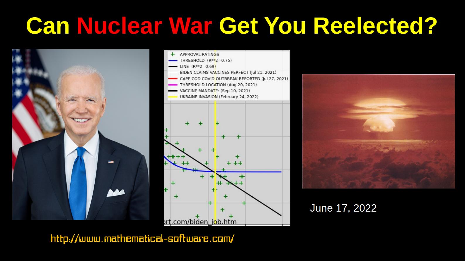
About twenty minute video on why the Manhattan Project, the World War II program that developed the first atomic bombs and reactors, is unusual among major inventions and discoveries both before and since. It was unusual in the number of major inventions and discoveries made in a few years and even more in that the first prototypes, the first full system tests (the Trinity bomb test in July 1945 and the bombings of Hiroshima and Nagasaki in August 1945) succeeded. Discusses the probable reason for this anomalous success and how it has led to inflated expectations for “New Manhattan Projects.”
Subscribe to our free Weekly Newsletter for articles and videos on practical mathematics, Internet Censorship, ways to fight back against censorship, and other topics by sending an email to: subscribe [at] mathematical-software.com
John F. McGowan, Ph.D. solves problems using mathematics and mathematical software, including developing gesture recognition for touch devices, video compression and speech recognition technologies. He has extensive experience developing software in C, C++, MATLAB, Python, Visual Basic and many other programming languages. He has been a Visiting Scholar at HP Labs developing computer vision algorithms and software for mobile devices. He has worked as a contractor at NASA Ames Research Center involved in the research and development of image and video processing algorithms and technology. He has published articles on the origin and evolution of life, the exploration of Mars (anticipating the discovery of methane on Mars), and cheap access to space. He has a Ph.D. in physics from the University of Illinois at Urbana-Champaign and a B.S. in physics from the California Institute of Technology (Caltech).
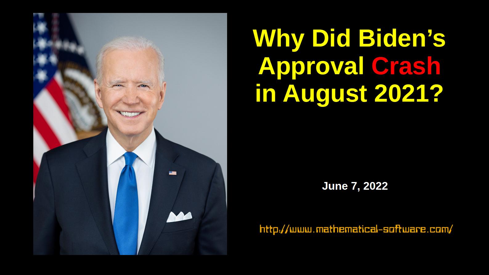
About twenty-minute (20) video on Operation Warp Speed and how inflated expectations from the extremely and unusually sucessful World War II Manhattan Project that produced the first atomic bombs contributed to grossly unrealistic expectations for the rapid development of COVID-19 vaccines. Discusses the lessons from the disappointing results of Operation Warp Speed and the frequent failure of other “New Manhatan Projects” (e.g. the War on Cancer) since World War II.
Subscribe to our free Weekly Newsletter for articles and videos on practical mathematics, Internet Censorship, ways to fight back against censorship, and other topics by sending an email to: subscribe [at] mathematical-software.com
John F. McGowan, Ph.D. solves problems using mathematics and mathematical software, including developing gesture recognition for touch devices, video compression and speech recognition technologies. He has extensive experience developing software in C, C++, MATLAB, Python, Visual Basic and many other programming languages. He has been a Visiting Scholar at HP Labs developing computer vision algorithms and software for mobile devices. He has worked as a contractor at NASA Ames Research Center involved in the research and development of image and video processing algorithms and technology. He has published articles on the origin and evolution of life, the exploration of Mars (anticipating the discovery of methane on Mars), and cheap access to space. He has a Ph.D. in physics from the University of Illinois at Urbana-Champaign and a B.S. in physics from the California Institute of Technology (Caltech).
This article takes a first look at historical Presidential approval ratings (approval polls from Gallup and other polling services) from Harry Truman through Joe Biden using our math recognition and automated model fitting technology. Our Math Recognition (MathRec) engine has a large, expanding database of known mathematics and uses AI and pattern recognition technology to identify likely candidate mathematical models for data such as the Presidential Approval ratings data. It then automatically fits these models to the data and provides a ranked list of models ordered by goodness of fit, usually the coefficient of determination or “R Squared” metric. It automates, speeds up, and increases the accuracy of data analysis — finding actionable predictive models for data.
The plots show a model — the blue lines — which “predicts” the approval rating based on unemployment rate (UNRATE), the real inflation adjusted value of gold, and time after the first inauguration of a US President — the so-called honeymoon period. The model “explains” about forty-three (43%) of the variation in the approval ratings. This is the “R Squared” or coefficient of determination for the model. The model has a correlation of about sixty-six percent (0.66) with the actual Presidential approval ratings. Note that a model can have a high correlation with data and yet the coefficient of determination is small.
One might expect US Presidential approval ratings to decline with increasing unemployment and/or an increase in the real value of gold reflecting uncertainty and anxiety over the economy. It is generally thought that new Presidents experience a honeymoon period after first taking office. This seems supported by the historical data, suggesting a honeymoon of about six months — with the possible exception of President Trump in 2017.
The model does not (yet) capture a number of notable historical events that appear to have significantly boosted or reduced the US Presidential approval ratings: the Cuban Missile crisis, the Iran Hostage Crisis, the September 11 attacks, the Watergate scandal, and several others. Public response to dramatic events such as these is variable and hard to predict or model. The public often seems to rally around the President at first and during the early stages of a war, but support may decline sharply as a war drags on and/or serious questions arise regarding the war.
There are, of course, a number of caveats on the data. Presidential approval polls empirically vary by several percentage points today between different polling services. There are several historical cases where pre-election polling predictions were grossly in error including the 2016 US Presidential election. A number of polls called the Dewey-Truman race in 1948 wrong, giving rise to the famous photo of President Truman holding up a copy of the Chicago Tribune announcing Dewey’s election victory.
The input data is from the St. Louis Federal Reserve Federal Reserve Economic Data (FRED) web site, much of it from various government agencies such as unemployment data from the Bureau of Labor Statistics. There is a history of criticism of these numbers. Unemployment and inflation rate numbers often seem lower than my everyday experience. As noted, a number of economists and others have questioned the validity of federal unemployment, inflation and price level, and other economic numbers.
(C) 2022 by John F. McGowan, Ph.D.
About Me
John F. McGowan, Ph.D. solves problems using mathematics and mathematical software, including developing gesture recognition for touch devices, video compression and speech recognition technologies. He has extensive experience developing software in C, C++, MATLAB, Python, Visual Basic and many other programming languages. He has been a Visiting Scholar at HP Labs developing computer vision algorithms and software for mobile devices. He has worked as a contractor at NASA Ames Research Center involved in the research and development of image and video processing algorithms and technology. He has published articles on the origin and evolution of life, the exploration of Mars (anticipating the discovery of methane on Mars), and cheap access to space. He has a Ph.D. in physics from the University of Illinois at Urbana-Champaign and a B.S. in physics from the California Institute of Technology (Caltech).
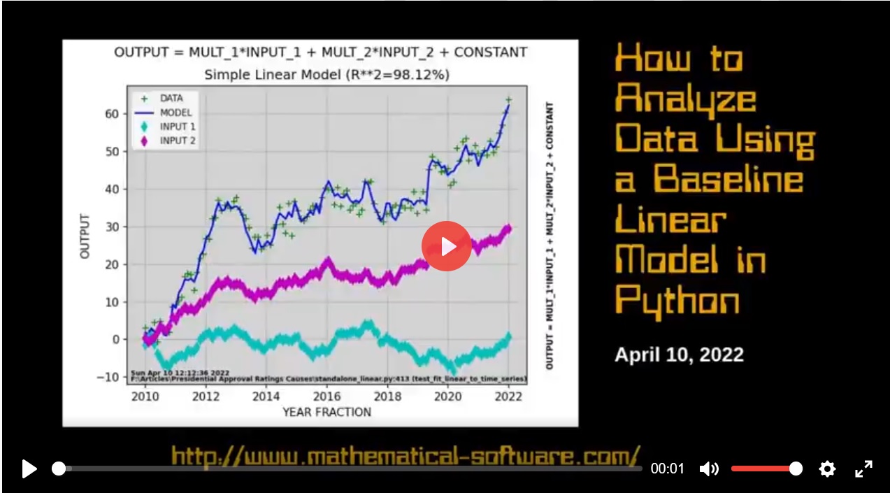
Video on how to analyze data using a baseline linear model in the Python programming language. A baseline linear model is often a good starting point, reference for developing and evaluating more advanced usually non-linear models of data.
John F. McGowan, Ph.D. solves problems using mathematics and mathematical software, including developing gesture recognition for touch devices, video compression and speech recognition technologies. He has extensive experience developing software in C, C++, MATLAB, Python, Visual Basic and many other programming languages. He has been a Visiting Scholar at HP Labs developing computer vision algorithms and software for mobile devices. He has worked as a contractor at NASA Ames Research Center involved in the research and development of image and video processing algorithms and technology. He has published articles on the origin and evolution of life, the exploration of Mars (anticipating the discovery of methane on Mars), and cheap access to space. He has a Ph.D. in physics from the University of Illinois at Urbana-Champaign and a B.S. in physics from the California Institute of Technology (Caltech).
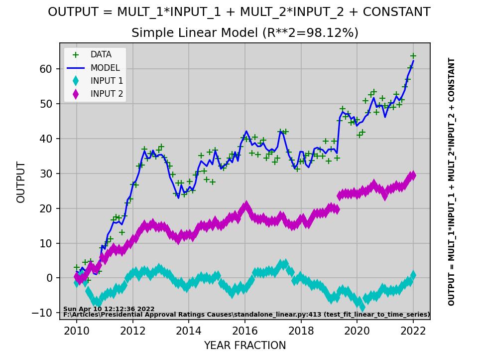
This article shows Python programming language source code to perform a simple linear model analysis of time series data. Most real world data is not linear but a linear model provides a common baseline starting point for comparison of more advanced, generally non-linear models.
"""
Standalone linear model example code.
Generate simulated data and fit model to this simulated data.
LINEAR MODEL FORMULA:
OUTPUT = MULT_T*DATE_TIME + MULT_1*INPUT_1 + MULT_2*INPUT_2 + CONSTANT + NOISE
set MULT_T to 0.0 for simulated data. Asterisk * means MULTIPLY
from grade school arithmetic. Python and most programming languages
use * to indicate ordinary multiplication.
(C) 2022 by Mathematical Software Inc.
Point of Contact (POC): John F. McGowan, Ph.D.
E-Mail: ceo@mathematical-software.com
"""
# Python Standard Library
import os
import sys
import time
import datetime
import traceback
import inspect
import glob
# Python add on modules
import numpy as np # NumPy
import pandas as pd # Python Data Analysis Library
import matplotlib.pyplot as plt # MATLAB style plotting
from sklearn.metrics import r2_score # scikit-learn
import statsmodels.api as sm # OLS etc.
# STATSMODELS
#
# statsmodels is a Python module that provides classes and functions for
# the estimation of many different statistical models, as well as for
# conducting statistical tests, and statistical data exploration. An
# extensive list of result statistics are available for each
# estimator. The results are tested against existing statistical
# packages to ensure that they are correct. The package is released
# under the open source Modified BSD (3-clause) license.
# The online documentation is hosted at statsmodels.org.
#
# statsmodels supports specifying models using R-style formulas and pandas DataFrames.
def debug_prefix(stack_index=0):
"""
return <file_name>:<line_number> (<function_name>)
REQUIRES: import inspect
"""
the_stack = inspect.stack()
lineno = the_stack[stack_index + 1].lineno
filename = the_stack[stack_index + 1].filename
function = the_stack[stack_index + 1].function
return (str(filename) + ":"
+ str(lineno)
+ " (" + str(function) + ") ") # debug_prefix()
def is_1d(array_np,
b_trace=False):
"""
check if array_np is 1-d array
Such as array_np.shape: (n,), (1,n), (n,1), (1,1,n) etc.
RETURNS: True or False
TESTING: Use DOS> python -c "from standalone_linear import *;test_is_1d()"
to test this function.
"""
if not isinstance(array_np, np.ndarray):
raise TypeError(debug_prefix() + "argument is type "
+ str(type(array_np))
+ " Expected np.ndarray")
if array_np.ndim == 1:
# array_np.shape == (n,)
return True
elif array_np.ndim > 1:
# (2,3,...)-d array
# with only one axis with more than one element
# such as array_np.shape == (n, 1) etc.
#
# NOTE: np.array.shape is a tuple (not a np.ndarray)
# tuple does not have a shape
#
if b_trace:
print("array_np.shape:", array_np.shape)
print("type(array_np.shape:",
type(array_np.shape))
temp = np.array(array_np.shape) # convert tuple to np.array
reference = np.ones(temp.shape, dtype=int)
if b_trace:
print("reference:", reference)
mask = np.zeros(temp.shape, dtype=bool)
for index, value in enumerate(temp):
if value == 1:
mask[index] = True
if b_trace:
print("mask:", mask)
# number of axes with one element
axes = temp[mask]
if isinstance(axes, np.ndarray):
n_ones = axes.size
else:
n_ones = axes
if n_ones >= (array_np.ndim - 1):
return True
else:
return False
# END is_1d(array_np)
def test_is_1d():
"""
test is_1d(array_np) function works
"""
assert is_1d(np.array([1, 2, 3]))
assert is_1d(np.array([[10, 20, 33.3]]))
assert is_1d(np.array([[1.0], [2.2], [3.34]]))
assert is_1d(np.array([[[1.0], [2.2], [3.3]]]))
assert not is_1d(np.array([[1.1, 2.2], [3.3, 4.4]]))
print(debug_prefix(), "PASSED")
# test_is_1d()
def is_time_column(column_np):
"""
check if column_np is consistent with a time step sequence
with uniform time steps. e.g. [0.0, 0.1, 0.2, 0.3,...]
ARGUMENT: column_np -- np.ndarray with sequence
RETURNS: True or False
"""
if not isinstance(column_np, np.ndarray):
raise TypeError(debug_prefix() + "argument is type "
+ str(type(column_np))
+ " Expected np.ndarray")
if is_1d(column_np):
# verify if time step sequence is nearly uniform
# sequence of time steps such as (0.0, 0.1, 0.2, ...)
#
delta_t = np.zeros(column_np.size-1)
for index, tval in enumerate(column_np.ravel()):
if index > 0:
previous_time = column_np[index-1]
if tval > previous_time:
delta_t[index-1] = tval - previous_time
else:
return False
# now check that time steps are almost the same
delta_t = np.median(delta_t)
delta_range = np.max(delta_t) - np.min(delta_t)
delta_pct = delta_range / delta_t
print(debug_prefix(),
"INFO: delta_pct is:", delta_pct, flush=True)
if delta_pct > 1e-6:
return False
else:
return True # steps are almost the same
else:
raise ValueError(debug_prefix() + "argument has more"
+ " than one (1) dimension. Expected 1-d")
# END is_time_column(array_np)
def validate_time_series(time_series):
"""
validate a time series NumPy array
Should be a 2-D NumPy array (np.ndarray) of float numbers
REQUIRES: import numpy as np
"""
if not isinstance(time_series, np.ndarray):
raise TypeError(debug_prefix(stack_index=1)
+ " time_series is type "
+ str(type(time_series))
+ " Expected np.ndarray")
if not time_series.ndim == 2:
raise TypeError(debug_prefix(stack_index=1)
+ " time_series.ndim is "
+ str(time_series.ndim)
+ " Expected two (2).")
for row in range(time_series.shape[0]):
for col in range(time_series.shape[1]):
value = time_series[row, col]
if not isinstance(value, np.float64):
raise TypeError(debug_prefix(stack_index=1)
+ "time_series[" + str(row)
+ ", " + str(col) + "] is type "
+ str(type(value))
+ " expected float.")
# check if first column is a sequence of nearly uniform time steps
#
if not is_time_column(time_series[:, 0]):
raise TypeError(debug_prefix(stack_index=1)
+ "time_series[:, 0] is not a "
+ "sequence of nearly uniform time steps.")
return True # validate_time_series(...)
def fit_linear_to_time_series(new_series):
"""
Fit multivariate linear model to data. A wrapper
for ordinary least squares (OLS). Include possibility
of direct linear dependence of the output on the date/time.
Mathematical formula:
output = MULT_T*DATE_TIME + MULT_1*INPUT_1 + ... + CONSTANT
ARGUMENTS: new_series -- np.ndarray with two dimensions
with multivariate time series.
Each column is a variable. The
first column is the date/time
as a float value, usually a
fractional year. Final column
is generally the suspected output
or dependent variable.
(time)(input_1)...(output)
RETURNS: fitted_series -- np.ndarray with two dimensions
and two columns: (date/time) (output
of fitted model)
results --
statsmodels.regression.linear_model.RegressionResults
REQUIRES: import numpy as np
import pandas as pd
import statsmodels.api as sm # OLS etc.
(C) 2022 by Mathematical Software Inc.
"""
validate_time_series(new_series)
#
# a data frame is a package for a set of numbers
# that includes key information such as column names,
# units etc.
#
input_data_df = pd.DataFrame(new_series[:, :-1])
input_data_df = sm.add_constant(input_data_df)
output_data_df = pd.DataFrame(new_series[:, -1])
# statsmodels Ordinary Least Squares (OLS)
model = sm.OLS(output_data_df, input_data_df)
results = model.fit() # fit linear model to the data
print(results.summary()) # print summary of results
# with fit parameters, goodness
# of fit statistics etc.
# compute fitted model values for comparison to data
#
fitted_values_df = results.predict(input_data_df)
fitted_series = np.vstack((new_series[:, 0],
fitted_values_df.values)).transpose()
assert fitted_series.shape[1] == 2, \
str(fitted_series.shape[1]) + " columns, expected two(2)."
validate_time_series(fitted_series)
return fitted_series, results # fit_linear_to_time_series(...)
def test_fit_linear_to_time_series():
"""
simple test of fitting a linear model to simple
simulated data.
ACTION: Displays plot comparing data to the linear model.
REQUIRES: import numpy as np
import matplotlib.pyplot as plt
from sklearn.metrics impor r2_score (scikit-learn)
NOTE: In mathematics a function f(x) is linear if:
f(x + y) = f(x) + f(y) # function of sum of two inputs
# is sum of function of each input value
f(a*x) = a*f(x) # function of constant multiplied by
# an input is the same constant
# multiplied by the function of the
# input value
(C) 2022 by Mathematical Software Inc.
"""
# simulate monthly data for years 2010 to 2021
time_steps = np.linspace(2010.0, 2022.0, 120)
#
# set random number generator "seed"
#
np.random.seed(375123) # make test reproducible
# make random walks for the input values
input_1 = np.cumsum(np.random.normal(size=time_steps.shape))
input_2 = np.cumsum(np.random.normal(size=time_steps.shape))
# often awe inspiring Greek letters (alpha, beta,...)
mult_1 = 1.0 # coefficient or multiplier for input_1
mult_2 = 2.0 # coefficient or multiplier for input_2
constant = 3.0 # constant value (sometimes "pedestal" or "offset")
# simple linear model
output = mult_1*input_1 + mult_2*input_2 + constant
# add some simulated noise
noise = np.random.normal(loc=0.0,
scale=2.0,
size=time_steps.shape)
output = output + noise
# bundle the series into a single multivariate time series
data_series = np.vstack((time_steps,
input_1,
input_2,
output)).transpose()
#
# np.vstack((array1, array2)) vertically stacks
# array1 on top of array 2:
#
# (array 1)
# (array 2)
#
# transpose() to convert rows to vertical columns
#
# data_series has rows:
# (date_time, input_1, input_2, output)
# ...
#
# the model fit will estimate the values for the
# linear model parameters MULT_T, MULT_1, and MULT_2
fitted_series, \
fit_results = fit_linear_to_time_series(data_series)
assert fitted_series.shape[1] == 2, "wrong number of columns"
model_output = fitted_series[:, 1].flatten()
#
# Is the model "good enough" for practical use?
#
# Compure R-SQUARED also known as R**2
# coefficient of determination, a goodness of fit measure
# roughly percent agreement between data and model
#
r2 = r2_score(output, # ground truth / data
model_output # predicted values
)
#
# Plot data and model predictions
#
model_str = "OUTPUT = MULT_1*INPUT_1 + MULT_2*INPUT_2 + CONSTANT"
f1 = plt.figure()
# set light gray background for plot
# must do this at start after plt.figure() call for some
# reason
#
ax = plt.axes() # get plot axes
ax.set_facecolor("lightgray") # confusingly use set_facecolor(...)
# plt.ylim((ylow, yhi)) # debug code
plt.plot(time_steps, output, 'g+', label='DATA')
plt.plot(time_steps, model_output, 'b-', label='MODEL')
plt.plot(time_steps, data_series[:, 1], 'cd', label='INPUT 1')
plt.plot(time_steps, data_series[:, 2], 'md', label='INPUT 2')
plt.suptitle(model_str)
plt.title(f"Simple Linear Model (R**2={100*r2:.2f}%)")
ax.text(1.05, 0.5,
model_str,
rotation=90, size=7, weight='bold',
ha='left', va='center', transform=ax.transAxes)
ax.text(0.01, 0.01,
debug_prefix(),
color='black',
weight='bold',
size=6,
transform=ax.transAxes)
ax.text(0.01, 0.03,
time.ctime(),
color='black',
weight='bold',
size=6,
transform=ax.transAxes)
plt.xlabel("YEAR FRACTION")
plt.ylabel("OUTPUT")
plt.legend(fontsize=8)
# add major grid lines
plt.grid()
plt.show()
image_file = "test_fit_linear_to_time_series.jpg"
if os.path.isfile(image_file):
print("WARNING: removing old image file:",
image_file)
os.remove(image_file)
f1.savefig(image_file,
dpi=150)
if os.path.isfile(image_file):
print("Wrote plot image to:",
image_file)
# END test_fit_linear_to_time_series()
if __name__ == "__main__":
# MAIN PROGRAM
test_fit_linear_to_time_series() # test linear model fit
print(debug_prefix(), time.ctime(), "ALL DONE!")
(C) 2022 by John F. McGowan, Ph.D.
About Me
John F. McGowan, Ph.D. solves problems using mathematics and mathematical software, including developing gesture recognition for touch devices, video compression and speech recognition technologies. He has extensive experience developing software in C, C++, MATLAB, Python, Visual Basic and many other programming languages. He has been a Visiting Scholar at HP Labs developing computer vision algorithms and software for mobile devices. He has worked as a contractor at NASA Ames Research Center involved in the research and development of image and video processing algorithms and technology. He has published articles on the origin and evolution of life, the exploration of Mars (anticipating the discovery of methane on Mars), and cheap access to space. He has a Ph.D. in physics from the University of Illinois at Urbana-Champaign and a B.S. in physics from the California Institute of Technology (Caltech).
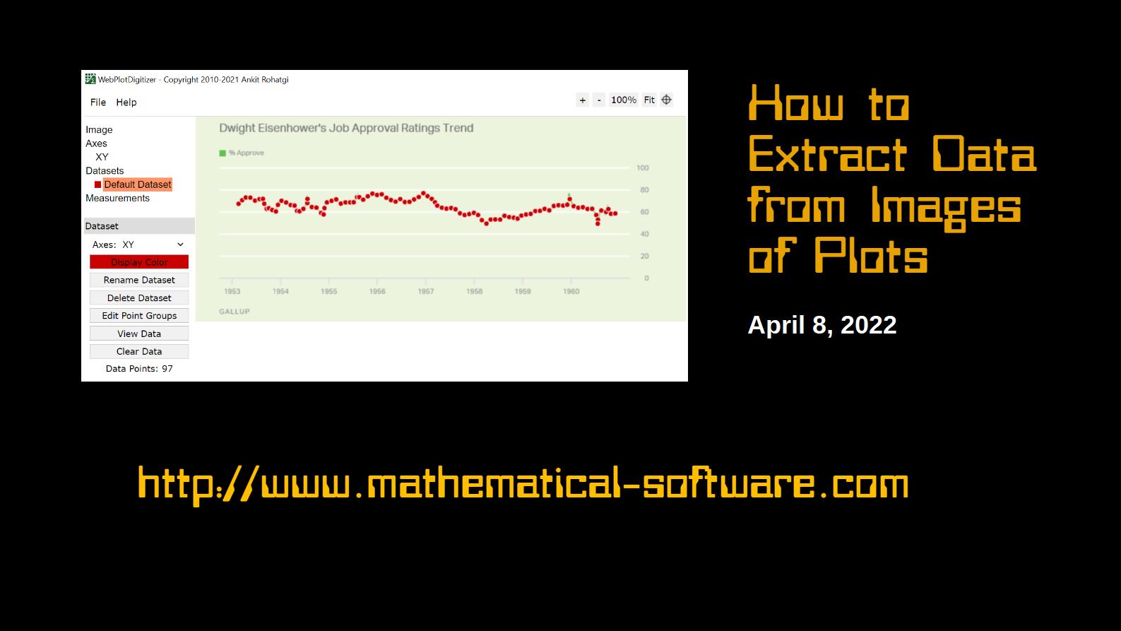
Short video on how to extract data from images of plots using WebPlotDigitizer, a free, open-source program available for Windows, Mac OS X, and Linux platforms.
John F. McGowan, Ph.D. solves problems using mathematics and mathematical software, including developing gesture recognition for touch devices, video compression and speech recognition technologies. He has extensive experience developing software in C, C++, MATLAB, Python, Visual Basic and many other programming languages. He has been a Visiting Scholar at HP Labs developing computer vision algorithms and software for mobile devices. He has worked as a contractor at NASA Ames Research Center involved in the research and development of image and video processing algorithms and technology. He has published articles on the origin and evolution of life, the exploration of Mars (anticipating the discovery of methane on Mars), and cheap access to space. He has a Ph.D. in physics from the University of Illinois at Urbana-Champaign and a B.S. in physics from the California Institute of Technology (Caltech).
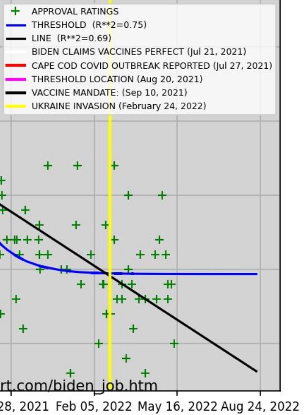
Short video discussing results of analyzing President Biden’s declining approval ratings and the possible effect of the COVID pandemic and Ukraine crises on the approval ratings.
A detailed longer explanation of the analysis discussed can be found in the previous video “How to Analyze Simple Data Using Python” available on all of our video channels.
(C) 2022 by John F. McGowan, Ph.D.
About Me
John F. McGowan, Ph.D. solves problems using mathematics and mathematical software, including developing gesture recognition for touch devices, video compression and speech recognition technologies. He has extensive experience developing software in C, C++, MATLAB, Python, Visual Basic and many other programming languages. He has been a Visiting Scholar at HP Labs developing computer vision algorithms and software for mobile devices. He has worked as a contractor at NASA Ames Research Center involved in the research and development of image and video processing algorithms and technology. He has published articles on the origin and evolution of life, the exploration of Mars (anticipating the discovery of methane on Mars), and cheap access to space. He has a Ph.D. in physics from the University of Illinois at Urbana-Champaign and a B.S. in physics from the California Institute of Technology (Caltech).
Video on how to analyze simple data using the Python programming language using President Biden’s approval ratings as an example.
(C) 2022 by John F. McGowan, Ph.D.
About Me
John F. McGowan, Ph.D. solves problems using mathematics and mathematical software, including developing gesture recognition for touch devices, video compression and speech recognition technologies. He has extensive experience developing software in C, C++, MATLAB, Python, Visual Basic and many other programming languages. He has been a Visiting Scholar at HP Labs developing computer vision algorithms and software for mobile devices. He has worked as a contractor at NASA Ames Research Center involved in the research and development of image and video processing algorithms and technology. He has published articles on the origin and evolution of life, the exploration of Mars (anticipating the discovery of methane on Mars), and cheap access to space. He has a Ph.D. in physics from the University of Illinois at Urbana-Champaign and a B.S. in physics from the California Institute of Technology (Caltech).