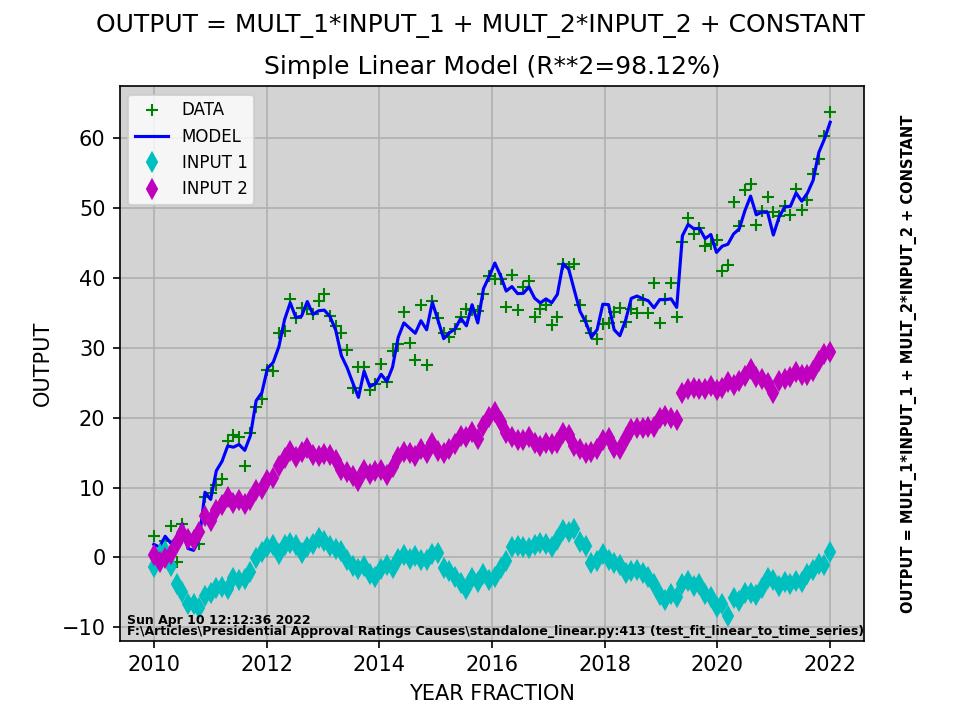
This article shows Python programming language source code to perform a simple linear model analysis of time series data. Most real world data is not linear but a linear model provides a common baseline starting point for comparison of more advanced, generally non-linear models.

"""
Standalone linear model example code.

Generate simulated data and fit model to this simulated data.

LINEAR MODEL FORMULA:

OUTPUT = MULT_T*DATE_TIME + MULT_1*INPUT_1 + MULT_2*INPUT_2 + CONSTANT + NOISE

set MULT_T to 0.0 for simulated data.  Asterisk * means MULTIPLY
from grade school arithmetic.  Python and most programming languages
use * to indicate ordinary multiplication.

(C) 2022 by Mathematical Software Inc.

Point of Contact (POC): John F. McGowan, Ph.D.
E-Mail: ceo@mathematical-software.com

"""

# Python Standard Library
import os
import sys
import time
import datetime
import traceback
import inspect
import glob
# Python add on modules
import numpy as np  # NumPy
import pandas as pd  # Python Data Analysis Library
import matplotlib.pyplot as plt  # MATLAB style plotting
from sklearn.metrics import r2_score  # scikit-learn
import statsmodels.api as sm  # OLS etc.

# STATSMODELS
#
# statsmodels is a Python module that provides classes and functions for
# the estimation of many different statistical models, as well as for
# conducting statistical tests, and statistical data exploration. An
# extensive list of result statistics are available for each
# estimator. The results are tested against existing statistical
# packages to ensure that they are correct. The package is released
# under the open source Modified BSD (3-clause) license.
# The online documentation is hosted at statsmodels.org.
#
# statsmodels supports specifying models using R-style formulas and pandas DataFrames.


def debug_prefix(stack_index=0):
    """
    return <file_name>:<line_number> (<function_name>)

    REQUIRES: import inspect
    """
    the_stack = inspect.stack()
    lineno = the_stack[stack_index + 1].lineno
    filename = the_stack[stack_index + 1].filename
    function = the_stack[stack_index + 1].function
    return (str(filename) + ":"
            + str(lineno)
            + " (" + str(function) + ") ")  # debug_prefix()


def is_1d(array_np,
          b_trace=False):
    """
    check if array_np is 1-d array

    Such as array_np.shape:  (n,), (1,n), (n,1), (1,1,n) etc.

    RETURNS: True or False

    TESTING: Use DOS> python -c "from standalone_linear import *;test_is_1d()"
    to test this function.

    """
    if not isinstance(array_np, np.ndarray):
        raise TypeError(debug_prefix() + "argument is type "
                        + str(type(array_np))
                        + " Expected np.ndarray")

    if array_np.ndim == 1:
        # array_np.shape == (n,)
        return True
    elif array_np.ndim > 1:
        # (2,3,...)-d array
        # with only one axis with more than one element
        # such as array_np.shape == (n, 1) etc.
        #
        # NOTE: np.array.shape is a tuple (not a np.ndarray)
        # tuple does not have a shape
        #
        if b_trace:
            print("array_np.shape:", array_np.shape)
            print("type(array_np.shape:",
                  type(array_np.shape))

        temp = np.array(array_np.shape)  # convert tuple to np.array
        reference = np.ones(temp.shape, dtype=int)

        if b_trace:
            print("reference:", reference)

        mask = np.zeros(temp.shape, dtype=bool)
        for index, value in enumerate(temp):
            if value == 1:
                mask[index] = True

        if b_trace:
            print("mask:", mask)

        # number of axes with one element
        axes = temp[mask]
        if isinstance(axes, np.ndarray):
            n_ones = axes.size
        else:
            n_ones = axes

        if n_ones >= (array_np.ndim - 1):
            return True
        else:
            return False
    # END is_1d(array_np)


def test_is_1d():
    """
    test is_1d(array_np) function  works
    """

    assert is_1d(np.array([1, 2, 3]))
    assert is_1d(np.array([[10, 20, 33.3]]))
    assert is_1d(np.array([[1.0], [2.2], [3.34]]))
    assert is_1d(np.array([[[1.0], [2.2], [3.3]]]))

    assert not is_1d(np.array([[1.1, 2.2], [3.3, 4.4]]))

    print(debug_prefix(), "PASSED")
    # test_is_1d()


def is_time_column(column_np):
    """
    check if column_np is consistent with a time step sequence
    with uniform time steps. e.g. [0.0, 0.1, 0.2, 0.3,...]

    ARGUMENT: column_np -- np.ndarray with sequence

    RETURNS: True or False
    """
    if not isinstance(column_np, np.ndarray):
        raise TypeError(debug_prefix() + "argument is type "
                        + str(type(column_np))
                        + " Expected np.ndarray")

    if is_1d(column_np):
        # verify if time step sequence is nearly uniform
        # sequence of time steps such as (0.0, 0.1, 0.2, ...)
        #
        delta_t = np.zeros(column_np.size-1)
        for index, tval in enumerate(column_np.ravel()):
            if index > 0:
                previous_time = column_np[index-1]
                if tval > previous_time:
                    delta_t[index-1] = tval - previous_time
                else:
                    return False

        # now check that time steps are almost the same
        delta_t = np.median(delta_t)
        delta_range = np.max(delta_t) - np.min(delta_t)
        delta_pct = delta_range / delta_t

        print(debug_prefix(),
              "INFO: delta_pct is:", delta_pct, flush=True)

        if delta_pct > 1e-6:
            return False
        else:
            return True  # steps are almost the same
    else:
        raise ValueError(debug_prefix() + "argument has more"
                         + " than one (1) dimension.  Expected 1-d")
    # END is_time_column(array_np)


def validate_time_series(time_series):
    """
    validate a time series NumPy array

    Should be a 2-D NumPy array (np.ndarray) of float numbers

    REQUIRES: import numpy as np

    """
    if not isinstance(time_series, np.ndarray):
        raise TypeError(debug_prefix(stack_index=1)
                        + " time_series is type "
                        + str(type(time_series))
                        + " Expected np.ndarray")

    if not time_series.ndim == 2:
        raise TypeError(debug_prefix(stack_index=1)
                        + " time_series.ndim is "
                        + str(time_series.ndim)
                        + " Expected two (2).")

    for row in range(time_series.shape[0]):
        for col in range(time_series.shape[1]):
            value = time_series[row, col]
            if not isinstance(value, np.float64):
                raise TypeError(debug_prefix(stack_index=1)
                                + "time_series[" + str(row)
                                + ", " + str(col) + "] is type "
                                + str(type(value))
                                + " expected float.")

    # check if first column is a sequence of nearly uniform time steps
    #
    if not is_time_column(time_series[:, 0]):
        raise TypeError(debug_prefix(stack_index=1)
                        + "time_series[:, 0] is not a "
                        + "sequence of nearly uniform time steps.")

    return True  # validate_time_series(...)


def fit_linear_to_time_series(new_series):
    """
    Fit multivariate linear model to data.  A wrapper
    for ordinary least squares (OLS).  Include possibility
    of direct linear dependence of the output on the date/time.
    Mathematical formula:

    output = MULT_T*DATE_TIME + MULT_1*INPUT_1 + ... + CONSTANT

    ARGUMENTS: new_series -- np.ndarray with two dimensions
                             with multivariate time series.
                             Each column is a variable.  The
                             first column is the date/time
                             as a float value, usually a
                             fractional year.  Final column
                             is generally the suspected output
                             or dependent variable.

                             (time)(input_1)...(output)

    RETURNS: fitted_series -- np.ndarray with two dimensions
                              and two columns: (date/time) (output
                              of fitted model)

             results --
                 statsmodels.regression.linear_model.RegressionResults

    REQUIRES: import numpy as np
              import pandas as pd
              import statsmodels.api as sm  # OLS etc.

    (C) 2022 by Mathematical Software Inc.

    """
    validate_time_series(new_series)

    #
    # a data frame is a package for a set of numbers
    # that includes key information such as column names,
    # units etc.
    #
    input_data_df = pd.DataFrame(new_series[:, :-1])
    input_data_df = sm.add_constant(input_data_df)

    output_data_df = pd.DataFrame(new_series[:, -1])

    # statsmodels Ordinary Least Squares (OLS)
    model = sm.OLS(output_data_df, input_data_df)
    results = model.fit()  # fit linear model to the data
    print(results.summary())  # print summary of results
                              # with fit parameters, goodness
                              # of fit statistics etc.

    # compute fitted model values for comparison to data
    #
    fitted_values_df = results.predict(input_data_df)

    fitted_series = np.vstack((new_series[:, 0],
                               fitted_values_df.values)).transpose()

    assert fitted_series.shape[1] == 2, \
        str(fitted_series.shape[1]) + " columns, expected two(2)."

    validate_time_series(fitted_series)

    return fitted_series, results  # fit_linear_to_time_series(...)


def test_fit_linear_to_time_series():
    """
    simple test of fitting  a linear model to simple
    simulated data.

    ACTION: Displays plot comparing data to the linear model.

    REQUIRES: import numpy as np
              import matplotlib.pyplot as plt
              from sklearn.metrics impor r2_score (scikit-learn)

    NOTE: In mathematics a function f(x) is linear if:

    f(x + y) = f(x) + f(y)  # function of sum of two inputs
                            # is sum of function of each input value

    f(a*x) = a*f(x)         # function of constant multiplied by
                            # an input is the same constant
                            # multiplied by the function of the
                            # input value

    (C) 2022 by Mathematical Software Inc.
    """

    # simulate monthly data for years 2010 to 2021
    time_steps = np.linspace(2010.0, 2022.0, 120)
    #
    # set random number generator "seed"
    #
    np.random.seed(375123)  # make test reproducible
    # make random walks for the input values
    input_1 = np.cumsum(np.random.normal(size=time_steps.shape))
    input_2 = np.cumsum(np.random.normal(size=time_steps.shape))

    # often awe inspiring Greek letters (alpha, beta,...)
    mult_1 = 1.0  # coefficient or multiplier for input_1
    mult_2 = 2.0   # coefficient or multiplier for input_2
    constant = 3.0  # constant value  (sometimes "pedestal" or "offset")

    # simple linear model
    output = mult_1*input_1 + mult_2*input_2 + constant
    # add some simulated noise
    noise = np.random.normal(loc=0.0,
                             scale=2.0,
                             size=time_steps.shape)

    output = output + noise

    # bundle the series into a single multivariate time series
    data_series = np.vstack((time_steps,
                             input_1,
                             input_2,
                             output)).transpose()

    #
    # np.vstack((array1, array2)) vertically stacks
    # array1 on top of array 2:
    #
    #  (array 1)
    #  (array 2)
    #
    # transpose() to convert rows to vertical columns
    #
    # data_series has rows:
    #    (date_time, input_1, input_2, output)
    #    ...
    #

    # the model fit will estimate the values for the
    # linear model parameters MULT_T, MULT_1, and MULT_2

    fitted_series, \
        fit_results = fit_linear_to_time_series(data_series)

    assert fitted_series.shape[1] == 2, "wrong number of columns"

    model_output = fitted_series[:, 1].flatten()

    #
    # Is the model "good enough" for practical use?
    #
    # Compure R-SQUARED also known as R**2
    # coefficient of determination, a goodness of fit measure
    # roughly percent agreement between data and model
    #
    r2 = r2_score(output,  # ground truth / data
                  model_output  # predicted values
                  )

    #
    # Plot data and model predictions
    #

    model_str = "OUTPUT = MULT_1*INPUT_1 + MULT_2*INPUT_2 + CONSTANT"

    f1 = plt.figure()
    # set light gray background for plot
    # must do this at start after plt.figure() call for some
    # reason
    #
    ax = plt.axes()  # get plot axes
    ax.set_facecolor("lightgray")  # confusingly use set_facecolor(...)
    # plt.ylim((ylow, yhi))  # debug code
    plt.plot(time_steps, output, 'g+', label='DATA')
    plt.plot(time_steps, model_output, 'b-', label='MODEL')
    plt.plot(time_steps, data_series[:, 1], 'cd', label='INPUT 1')
    plt.plot(time_steps, data_series[:, 2], 'md', label='INPUT 2')
    plt.suptitle(model_str)
    plt.title(f"Simple Linear Model (R**2={100*r2:.2f}%)")

    ax.text(1.05, 0.5,
            model_str,
            rotation=90, size=7, weight='bold',
            ha='left', va='center', transform=ax.transAxes)

    ax.text(0.01, 0.01,
            debug_prefix(),
            color='black',
            weight='bold',
            size=6,
            transform=ax.transAxes)

    ax.text(0.01, 0.03,
            time.ctime(),
            color='black',
            weight='bold',
            size=6,
            transform=ax.transAxes)

    plt.xlabel("YEAR FRACTION")
    plt.ylabel("OUTPUT")
    plt.legend(fontsize=8)
    # add major grid lines
    plt.grid()
    plt.show()

    image_file = "test_fit_linear_to_time_series.jpg"
    if os.path.isfile(image_file):
        print("WARNING: removing old image file:",
              image_file)
        os.remove(image_file)

    f1.savefig(image_file,
               dpi=150)

    if os.path.isfile(image_file):
        print("Wrote plot image to:",
              image_file)

    # END test_fit_linear_to_time_series()


if __name__ == "__main__":
    # MAIN PROGRAM

    test_fit_linear_to_time_series()  # test linear model fit

    print(debug_prefix(), time.ctime(), "ALL DONE!")
(C) 2022 by John F. McGowan, Ph.D.
About Me
John F. McGowan, Ph.D. solves problems using mathematics and mathematical software, including developing gesture recognition for touch devices, video compression and speech recognition technologies. He has extensive experience developing software in C, C++, MATLAB, Python, Visual Basic and many other programming languages. He has been a Visiting Scholar at HP Labs developing computer vision algorithms and software for mobile devices. He has worked as a contractor at NASA Ames Research Center involved in the research and development of image and video processing algorithms and technology. He has published articles on the origin and evolution of life, the exploration of Mars (anticipating the discovery of methane on Mars), and cheap access to space. He has a Ph.D. in physics from the University of Illinois at Urbana-Champaign and a B.S. in physics from the California Institute of Technology (Caltech).
